Contact Michal Tykac for more information.

Contents:

• Summary
• Re-boxing maps
• ... How the re-boxing works
• ... How to use re-boxing
• Shape-distance computation
• ... How the shape-distance computation works
• ... How to use shape-distance computation
• Symmetry detection
• ... How the symmetry detection works
• ... How to use the symmetry detection
• Structure overlay
• ... How the structure overlay works
• ... How to use the structure overlay

Summary:

ProSHADE (Proitein SHApe DEscription and symmetry detection) is a library and an associated tool providing functionalities for working with structural biology molecular structures. The library implements functions for computing shape-wise structural distances between pairs of molecules, detecting symmetry over the centre of mass of a single structure, map re-sizing as well as matching density maps and PDB coordinate files into one another. ProSHADE is avaialbe as a Linux/Mac executable, a C++ language library or as a Python language module.

In this tutorial, the use of the exetable is assumed, but the same functionality is available through the C++ library and Python module, albeit this does require a little more programming knowledge and allows for programmatical access to the results.

Map Re-boxing:

This functionality is not available for co-ordinate data.

How the re-boxing works:

This functionality comes from the observation that most maps are placed in a box much larger than required by the density. While this has generally advantage as it leads to oversampling in the reciprocal space, it also leads to increased cost of processing the map data, be it for visualisation or any other purposes.

Therefore, ProSHADE will increase the blurring of the map by a factor stated by the --mapMaskBlur argument and subsequently use the number of interquartile ranges given by the --mapMaskThres argument to modify the blurred map into a mask; any map value under this threshold will be set to 0, while any value above the threshold will be set to 1. With this mask computed, ProSHADE will take the minimal dimensions required to keep all mask values 1 and creates a new, empty map with these dimensions. Finally, the exect data from the original map within these dimensions will be copied to the new map and the new map will be saved as output. Therefore, there is no change in the map values for the retained box, but all data outside this box will be lost.

How to use re-boxing:

In order to run the re-boxing functionality of ProSHADE, the following example map will be used: EMD_1290 (Wyatt K, White HE, Wang L, Bateman OA, Slingsby C, Orlova EV and Wistow G (2006) Lengsin is a survivor of an ancient family of class I glutamine synthetases re-engineered by evolution for a role in the vertebrate lens. STRUCTURE 14, pp. 1823-1834)

Now, to invoke the re-boxing functionality, the -E option needs to be supplied as well as the path to the map which is to be re-boxed preceded by the -f argument. The output will be by default written into a file named proshade_reboxed.map, but the argument --clearMap can be used to supply a different name. Finally, the two command line arguments mentioned above, namely --mapMaskBlur and --mapMaskThres can be used to override the default values.

Therefore, a ProSHADE re-boxing run can be accomplished by entering

proshade -E -f EMD_1290.map

command. Alternatively, the user can customise the run by using the command line arguments as follows:

proshade -E -f EMD_1290.map --clearMap res.map --mapMaskBlur 500 --mapMaskThres 3.0

The resulting file will contain the re-boxed map, which can be used for further data analysis and processing. The following screenshot shows the result for the test map EMD_1290.

Shape-distance computation:

This functionality is available for both map and co-ordinate data.

How the shape-distance computation works:

This functionality is the workhorse of ProSHADE and consists of three different shape descriptors. All of the descriptors are based on spherical harmonics expansion performed on a set of concentric spheres with different radii placed into the expanded structure data. For more details about the procedure and the mathematical background for these descriptors, please see the accompanying doctoral thesis.

Therefore, ProSHADE will take two or more files (both co-ordinate and map files are allowed) and proceed to expand these files into a series of spherical harmonics coefficients. Then, using these coefficients, it will compute how similar the first input file is to all other input files. Please note that ProSHADE will not compute the full distance matrix for all input files. Generally, the energy level descriptor values are the least reliable, but the fastest to compute and these values reflect the similarity in terms of the correlation of the spherical harmonics coefficients between various spheres mentioned above. The trace sigma descriptor values take a bit longer to compute, but are more reliable; these values reflect the similarity in terms of the spherical harmonics coefficients distance for objects rotationally aligned using simplified SVD approach. Finally, the rotation function distance is the similarity in terms of spherical harmonics coefficients for objects rotationally aligned using the rotation function search. This approach takes the longest to compute, but is the most reliable.

All three descriptors are normalised so that the value of 1.0 signifies complete identity of the two objects, while the value of 0.0 means the object are completely dissimilar and the value of -1.0 would signify a complete "oppositeness" in terms of shape.

How to use shape-distance computation:

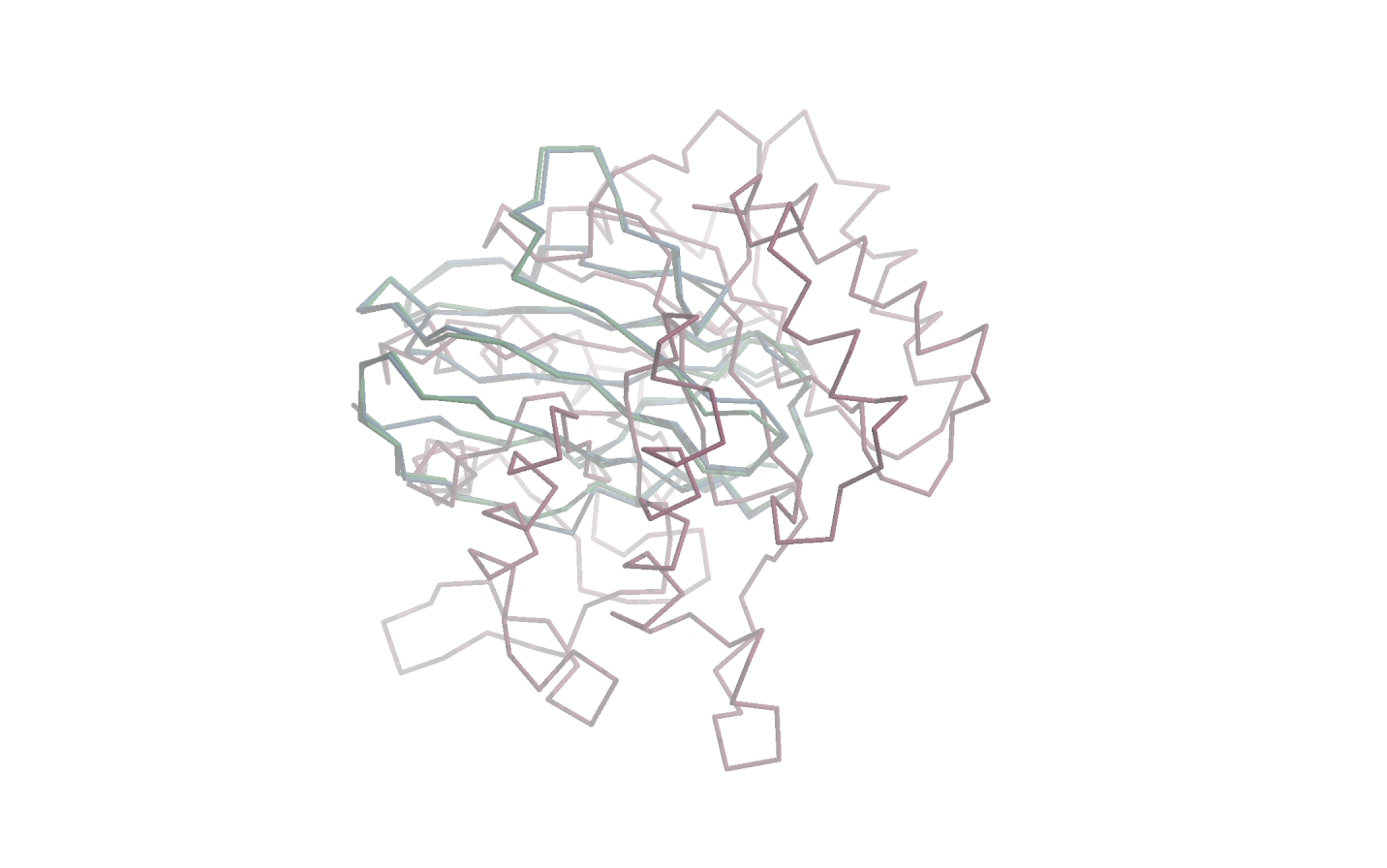
The shape-distance computation will be demonstrated usingg the following protein domain files from the BALBES (F. Long, A. A. Vagin, P. Young and G. N. Murshudov (2008) BALBES: a molecular-replacement pipeline. Acta Cryst. D64, pp. 125-132)

These three protein domains are visualised on the following figure with the 1BFO_A_dom_1 being shown in green, 1H8N_A_dom_1 in blue and 3IGU_A_dom_1 in red. This visualisation should demonstrate that the first two protein domains (green and blue) are very similar in terms of shape, while the third domain (red) is very dissimilar to both of the other two domains.

With the files available, proshade can now be used to obtain the distance between them by invoking the following command:

Where the -D option now states that distances are to be computed and the -f arguments precede each input file path. There are many optional command line options which can be used to customise the ProSHADE run to fit the users particular purposes. Some of the useful command line options are described below:

Symmetry detection:

This functionality is available for both map and co-ordinate data.

How the symmetry detection works:

The symmetry detection makes use of the inverse SO(3) Fourier Transform (SOFT) procedure to compute the rotation function for a given object against itself. A detailed description of this procedure can be found in the SOFT2.0 software documentation and the accompanying paper (P. J. Kostelec and D. N. Rockmore (2008) FFTs on the Rotation Group. J. Fourier Anal. Appl. 14, pp. 145-179). Nonetheless, the result of applying this procedure to a structure is a three-dimensional map with its dimensions being the three Euler angles α, β and γ. The values in this map are then the correlation values between the structure and its copy rotated by the Euler angles given by the axes. An example of such a map can be seen in the following figure for a structure with C12 symmetry.

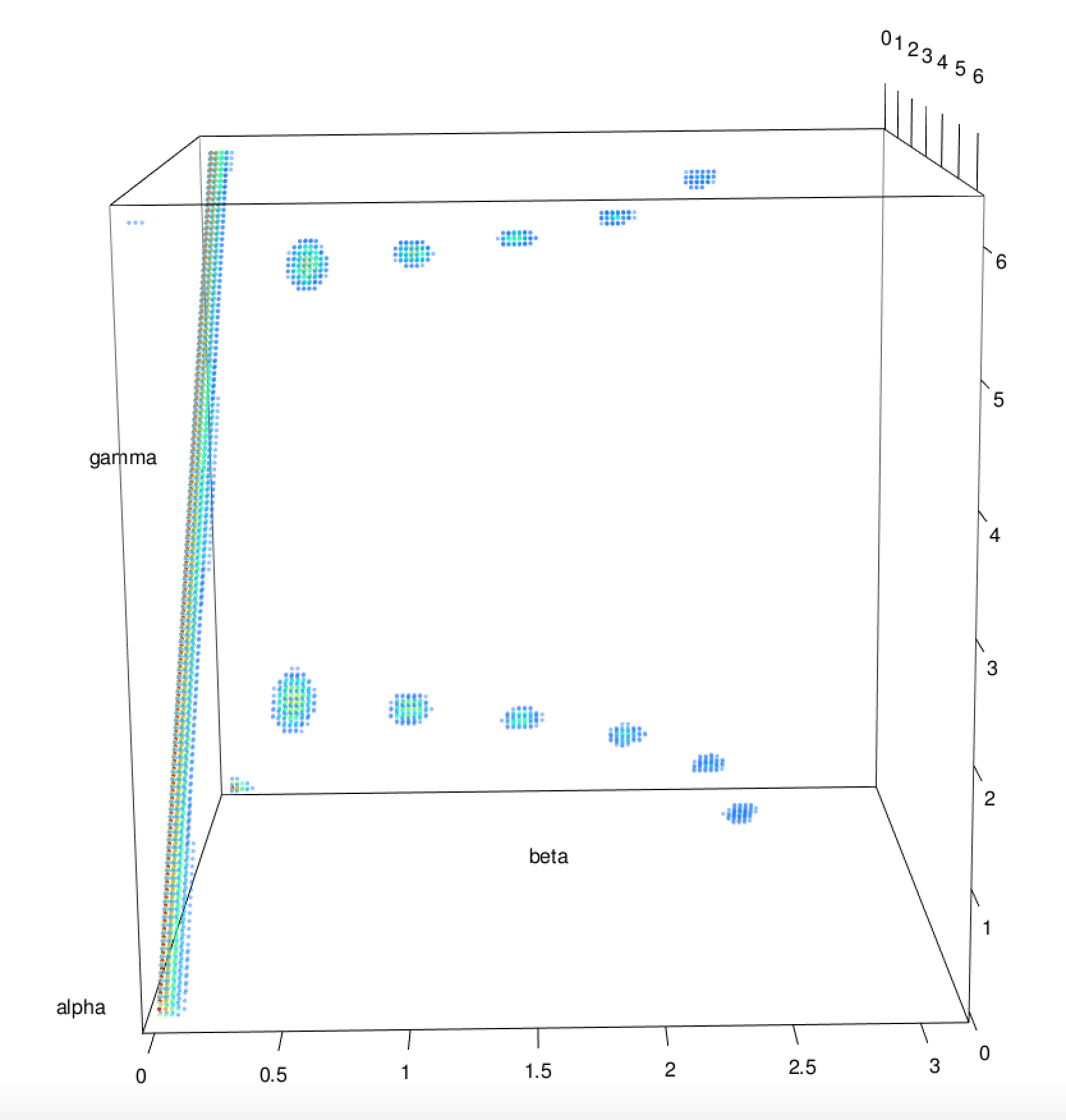
Therefore, any high peaks is this map will correspond to rotations over the centre which do not change the shape considerably, a condition which does define shape symmetry. Subsequently, the positions and heights of these peaks can be used to determine any cyclic symmetries, which can in turn be used to detect any dihedral, tetrahedral, otahedral and icosahedral symmetries.

How to use the symmetry detection:

The symmetry detection can be demonstrated on the same map file as was used to the re-boxing part, i.e. EMD_1290.

In order to make ProSHADE process the file for symmetry, it needs to be called using the following command:

Which will result in several tables being printed for the user. The first table contains the list of symmetries that ProSHADE believes to be the correct shape symmetry for the input file, as well as the axes and their associated angles for these symmetries and the average height of the peaks that resulted in this symmetry being detected. The second table contains all the symmetry elements (i.e. individual rotations) associated with the symmetry, while the last table contains the alternative symmetries, which were also detected in the shape - these are typically the sub-groups of the reported symmetry group.

The main command line argument of interest for the symmetry detection functionality is the --sym argument, which allows the user to specify which symmetry they believe the file contains and push ProSHADE to search specifically for this symmetry. The symmetry type is entered by first using the symmetry type letter (C = cyclic, D = dihedral, T = tetrahedral, O = octahedral and I = icosahedral) and then using a number to specify the fold, if appropriate (i.e. for cyclic and dihedral symmetry types). A request for D4 symmetry would, therefore, look like --sym D4.

There are several further command line options available to customise the ProSHADE run as listed below:

Structure overlay:

This functionality is available for both map and co-ordinate data.

How the structure overlay works:

This functionality makes use the ProSHADE internal structure representation, which is always a map-like array. This allows for the phase information to be removed from the map representation by performing forward Fourier transform, setting the phase to 0.0 and performing the inverse Fourier transform on the resulting map. Consequently, the Patterson maps can be expanded in spherical harmonics coefficients and subjected to the SOFT transformation (discussed above for the symmetry detection part). The resulting rotation function map then leads to determining the ideal rotation in terms of the correlation between the Patterson functions of the two input structure.

Once this rotation is applied to the original phased data, the translation function can be used to find the optimal translation required to maximise the correlation between the two structures; once the translation is applied, the two input structures are considered optimally overlayed by ProSHADE and the moving structure is outputted for visualisation of the overlay. It is worth noting that while this approach does a global search in terms of both translation and rotation, and therefore should not be sensitive to local minima, it does not do optimisation and therefore there are errors resulting from the coarseness of the rotation and translation function sampling.

Furthermore, it should be noted that the structure overlay computation tries to match the shapes completely and does not deal with one shape being a subset of the other. Therefore, if you are attempting to match a domain to a complete map, this procedure will not produce the optimal result.

How to use the structure overlay:

The structure overlay mode will be demonstrated using the following two files; where the co-ordinate file is a domain from the BALBES protein domain database and the map file was produced by computing the theoretical density map from this co-ordinate file.

Using these two files, the ProSHADE command required to move the moving structure to match the static structure is as follows:

This command will result in two files being saved into the current directory, one baing the res.pdb and the other being the res.map. Both these files will contain a rotated and translated version of the moving structure, one the co-ordinates and the other the internal ProSHADE map representation. Note that if the order of input files were reversed (i.e. map was fitted to co-ordinates), the res.pdb file would not be produced.

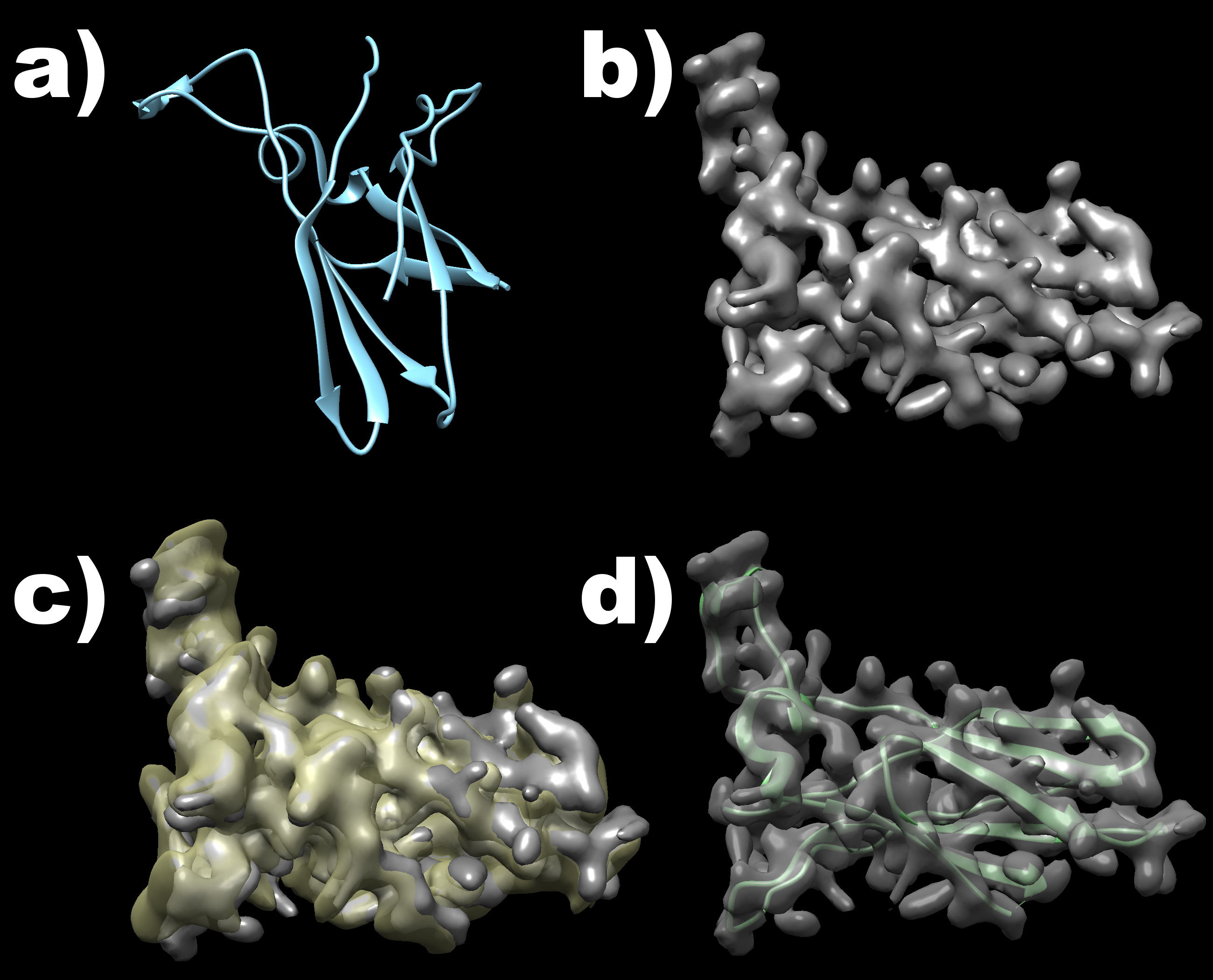
Visualisation of the example structures as well as their overlay is shown in the following image. The original structure is shown in part a), while a density map computed with low resolution from this structure is shown in part b). Part c) then shows the match obteined by the internal map representations of both inputs, while part d) shows the final match of the moved PDB file to the original map input.

Finally, there are some command line options the user can find useful when customising the ProSHADE execution to their particular purposes.