Creating Figures with Coot 1.1
Lucrezia Catapano - April 2025
Introduction
The Coot 1.1 graphics has been improved to the point of being useful
for publication.
This tutorial will explain how to make
high-quality figures of molecular models and maps with Coot 1.1.
1. Model Representations
Open Coot 1.1 and load a PDB file :
- File → Fetch PDB using Accession Code
- Enter 7P9B and click Get Structure
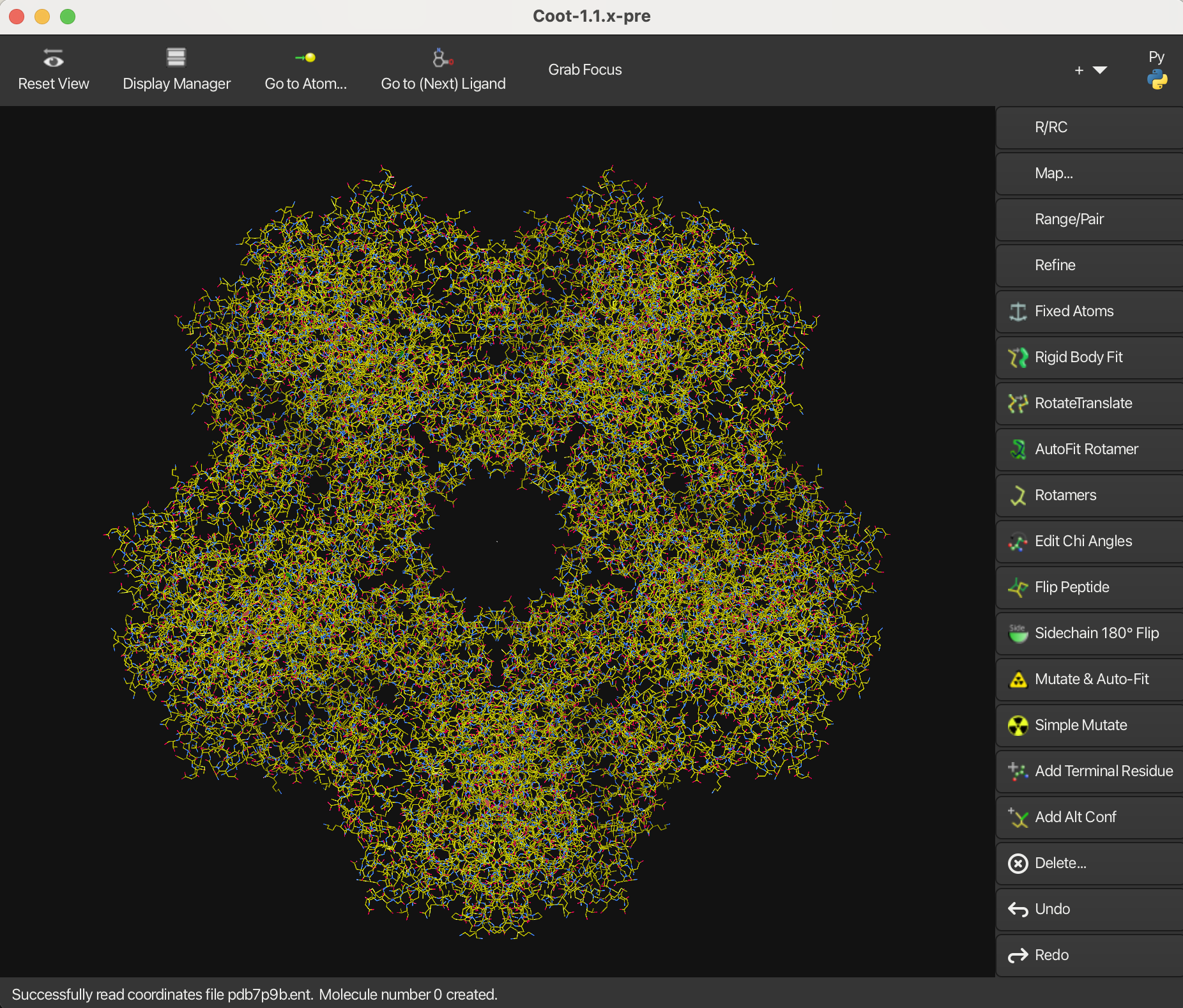
1.1 Bonds (Sticks)
Bonds are the default representation in Coot. To zoom in, hold Shift and use the Left Mouse Button. To center on a specific residue, press Ctrl G, type A7, and click OK.
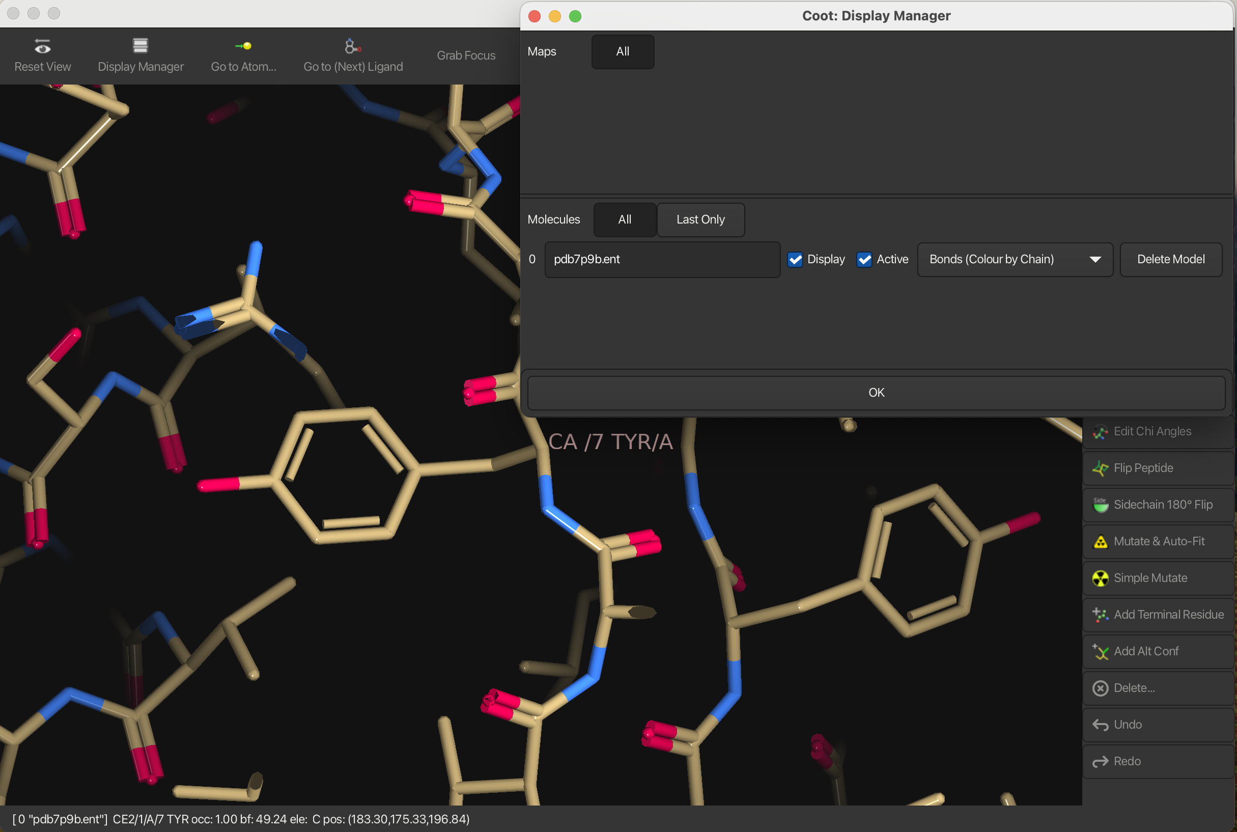
Let’s display bond orders for the molecule (coot uses a kekulised representation):
- Open the Display Manager on the toolbar
- in the Molecule window, select Bonds (Colour by chain)
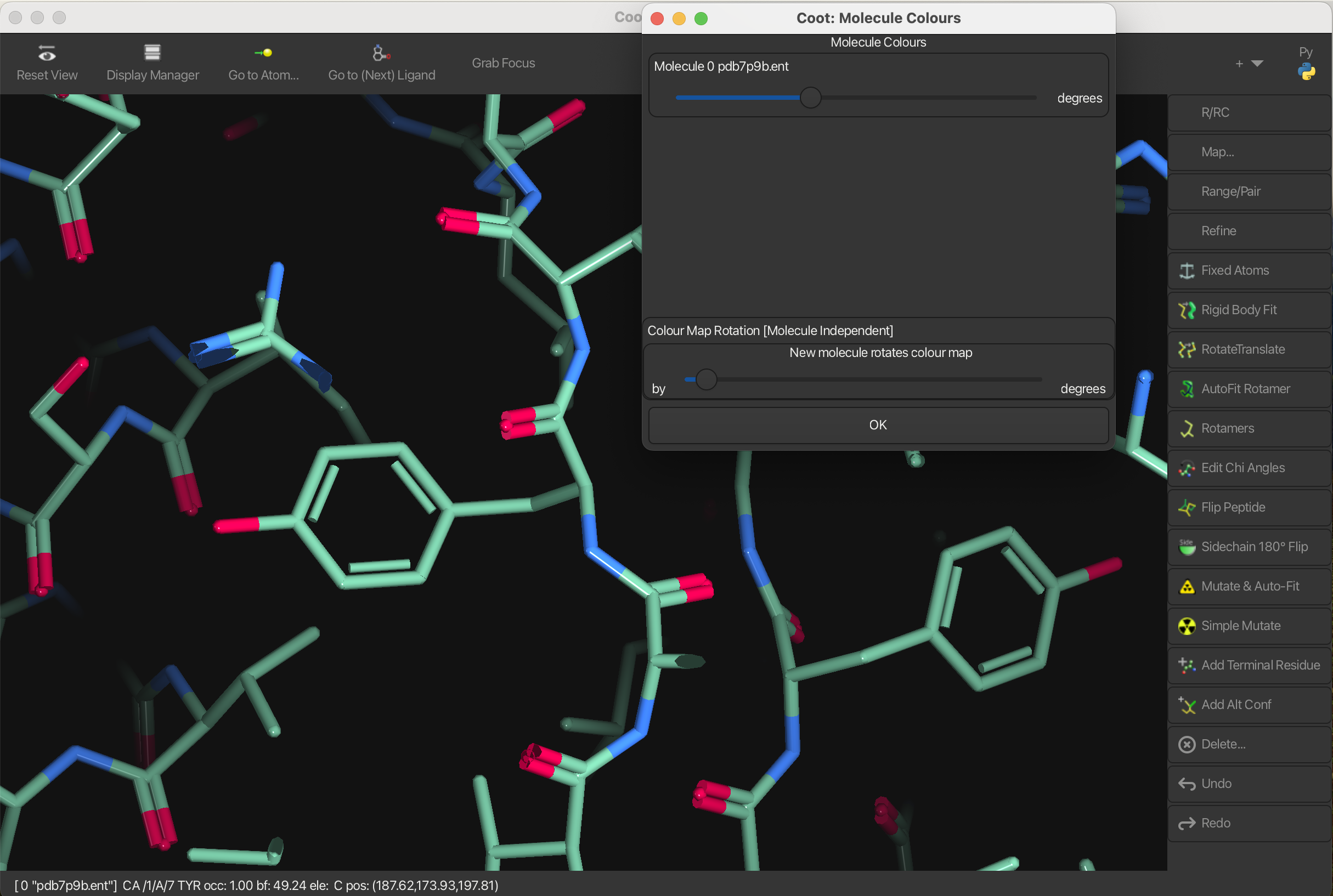
Colors
To change the colors of the bonds:
- Go to Draw → Molecule → Bond Colours.
- Use the color picker or slider to adjust the bond colors as desired.
Width
To change the width of the bonds:
- Go to Draw → Molecule → Bond Parameters.
- Change the pixels in Molecule Bond Width to 8.0 to make the bonds thicker.
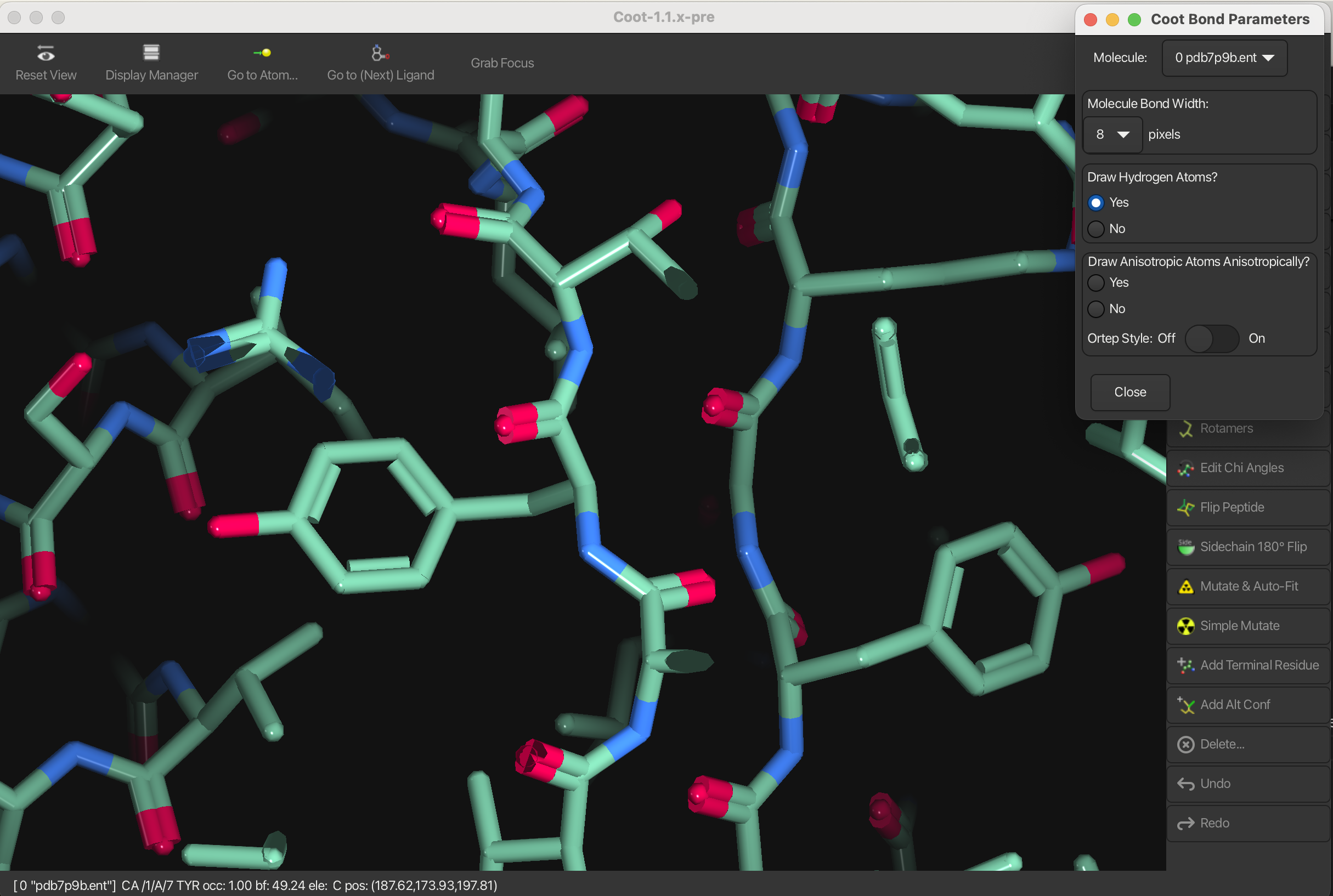
You can also change the smoothness of the bonds by selecting Bond Smoothness
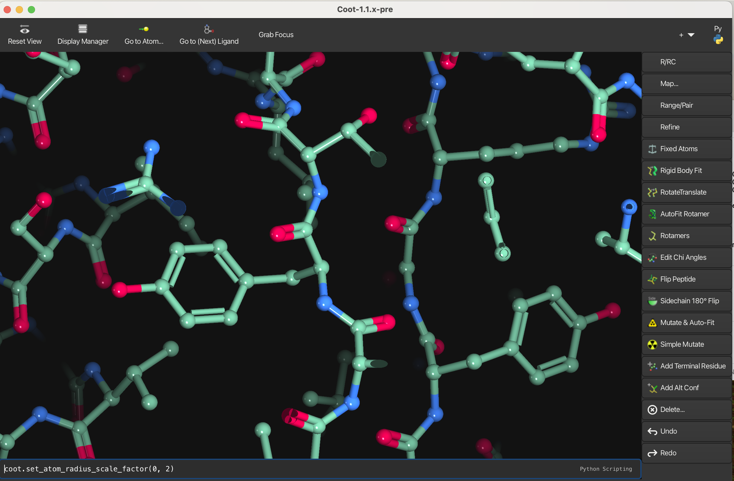
1.2 Ball and Stick
To create a ball and stick representation:
Click the Py button on the right-hand side of the horizontal toolbar to open the Python console (at the bottom).
Type the following commands and press Enter after each:
- import coot
- coot.set_atom_radius_scale_factor(0, 2.0) # Adjusts the atom radius scale factor
- coot.set_bond_smoothness_factor(3) # Increases the smoothness of the balls
- Note: Replace
0with the molecule index as shown in the Display Manager if needed.
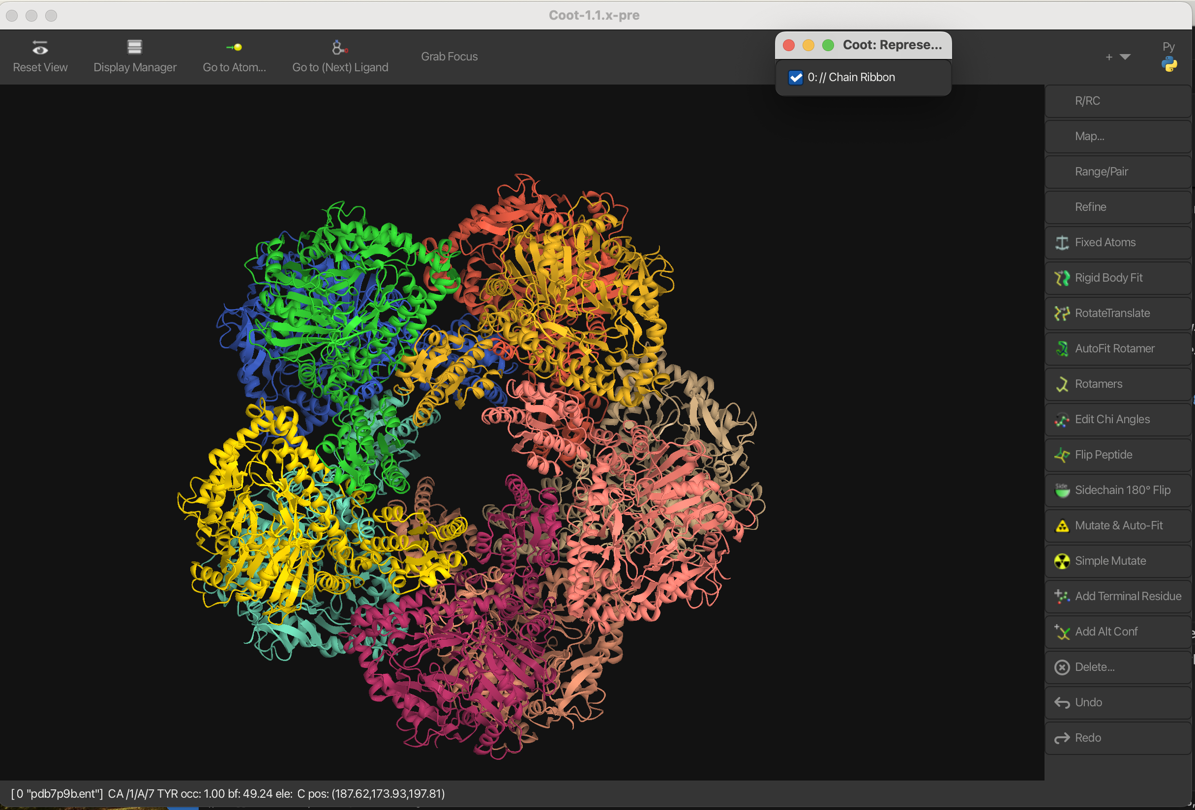
1.3 Ribbons
To create a ribbon representation:
- Navigate to Draw → Molecule → Ribbons: By Chain. A small window will appear.
- In the Display Manager, undisplay the model to disable the bond representation.
You can also enable the Ribbons: Rainbow and Ribbons: Sec. Struct. representations.
1.4 Molecular Surface
To create a molecular surface representation:
- Navigate to Draw → Molecule → Molecular Surface.
To undisplay the molecular surface:
- Go to Draw → View → Generic Display Objects.
- Either uncheck the molecular surface or click Delete All Generic Display Objects to remove all generic objects from the view.
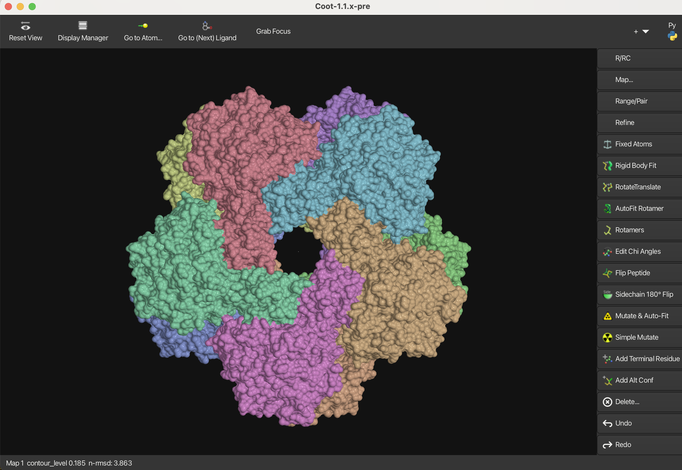
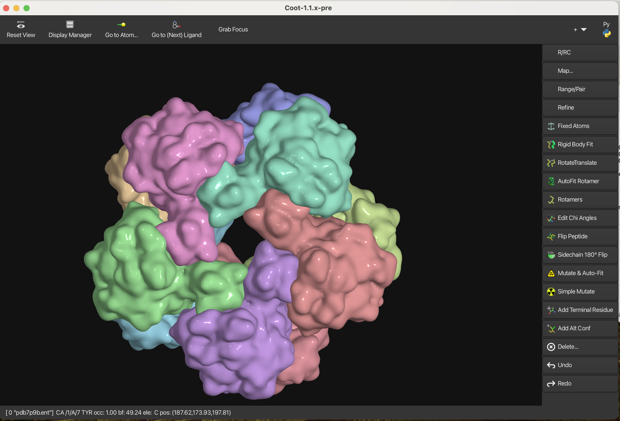
1.5 Gaussian Surface
To create a Gaussian surface representation:
- Navigate to Draw → Molecule → Gaussian Surface.
- In the window that appears, adjust the parameters as needed to customize the surface.
- Click Calculate to generate the Gaussian surface.
To undisplay the Gaussian surface:
- Go to Draw → View → Generic Display Objects.
- Either uncheck the Gaussian surface or click Delete All Generic Display Objects to remove all generic objects from the view.
1.6 Electrostatic Surface
To create an electrostatic surface representation:
- Navigate to Draw → Molecule → Electrostatic Surface.
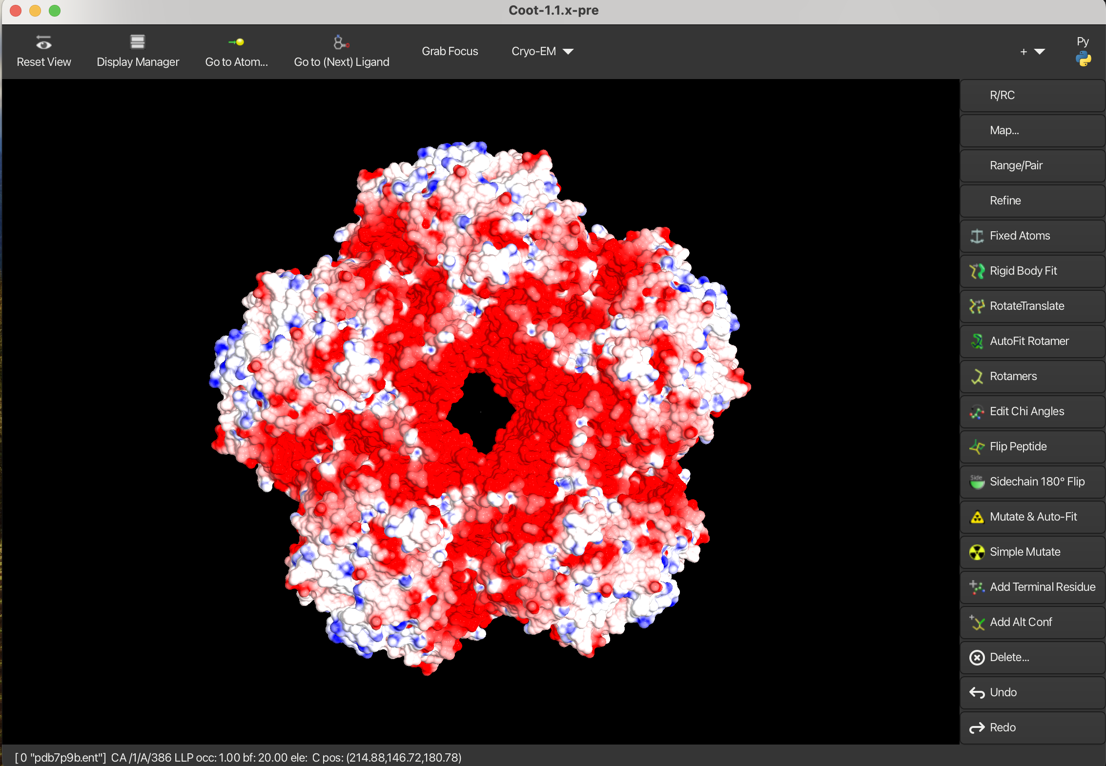
To undisplay the electrostatic surface:
- Go to Draw → View → Generic Display Objects.
- Either uncheck the electrostatic surface or click Delete All Generic Display Objects to remove all generic objects from the view.
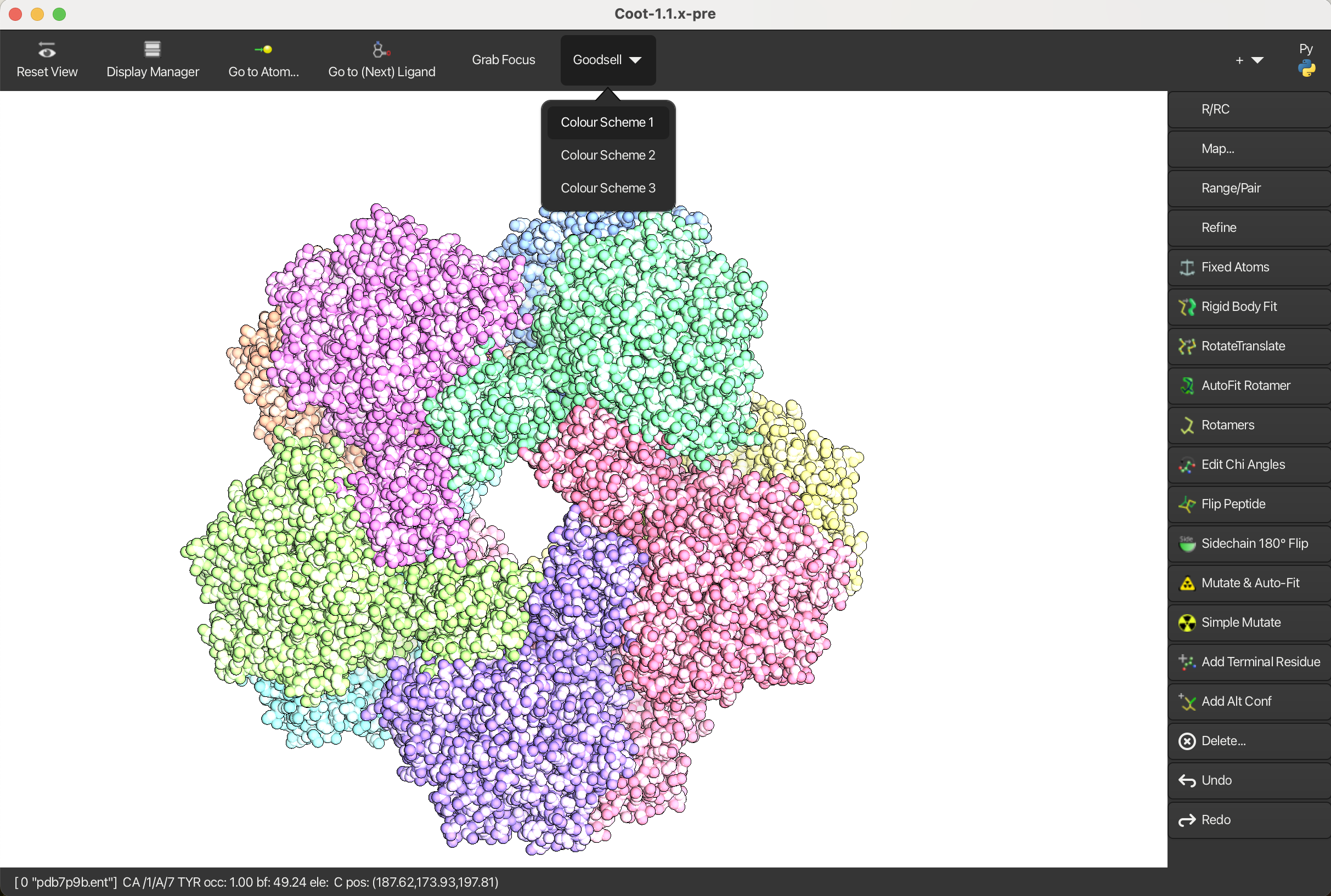
1.7 Goodsell Style
To enable Goodsell style:
- Go to File → Curlew and install the Goodsell Menu
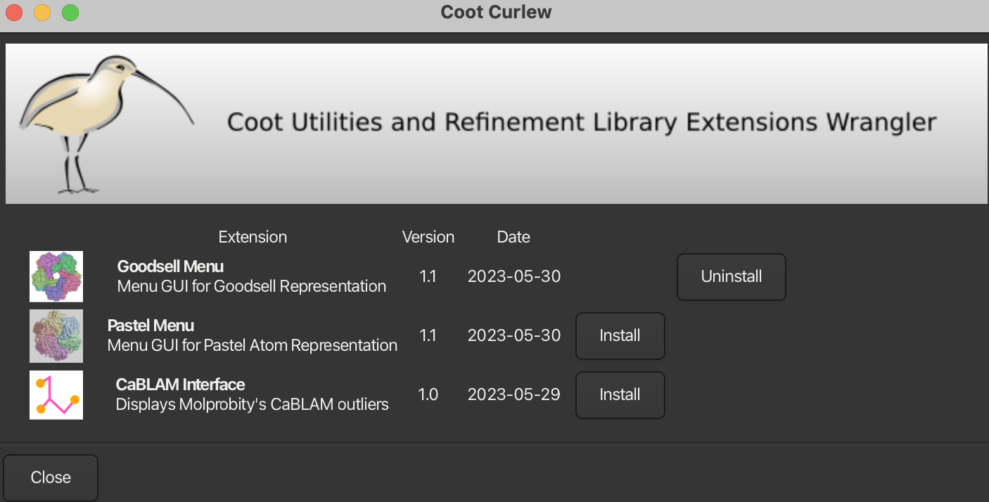
Then a Goodsell menu will appear on the horizontal toolbar.
The Goodsell representation offers three color schemes and the background colour is white by default.
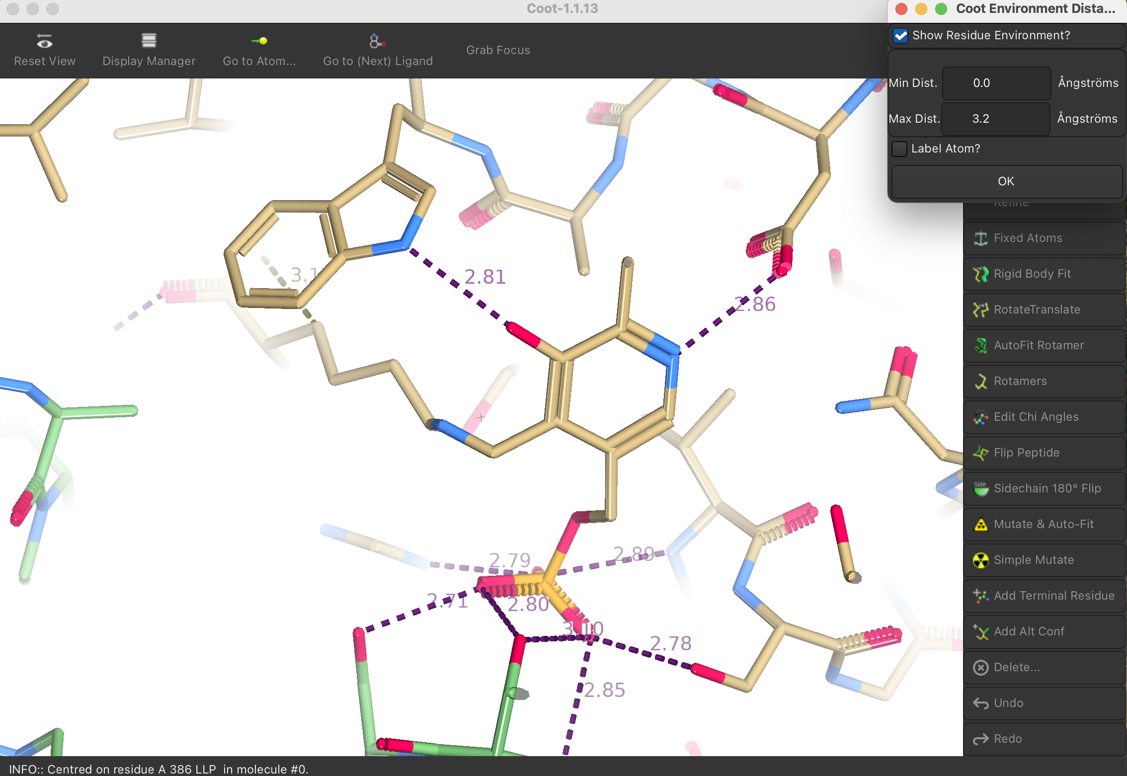
1.8 Environment Distances
To display environment distances:
- Navigate to Measures → Environment Distances. A
small window will appear.
- Check Show Residue Environment
- Purple dashed lines represent hydrogen bonds, while yellow lines indicate bumps.
2. Map Representation
Let’s load the map for 7p9b:
- File → Open Map
- Upload emd_13261.map and click Open.
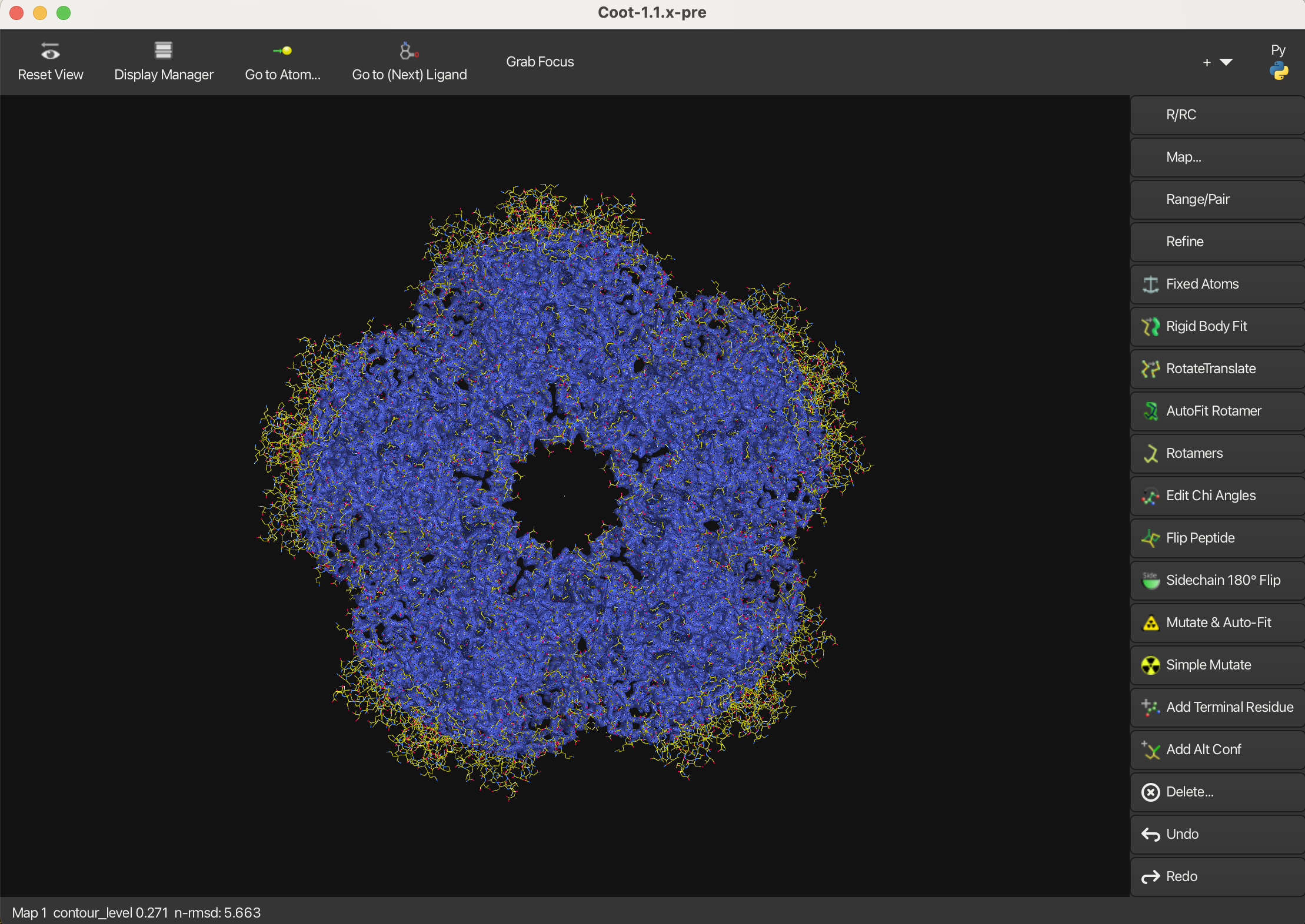
2.1 Chickenwire
The default representation of the map is a chickenwire.
To increase the contour level, use the mouse scroll wheel.
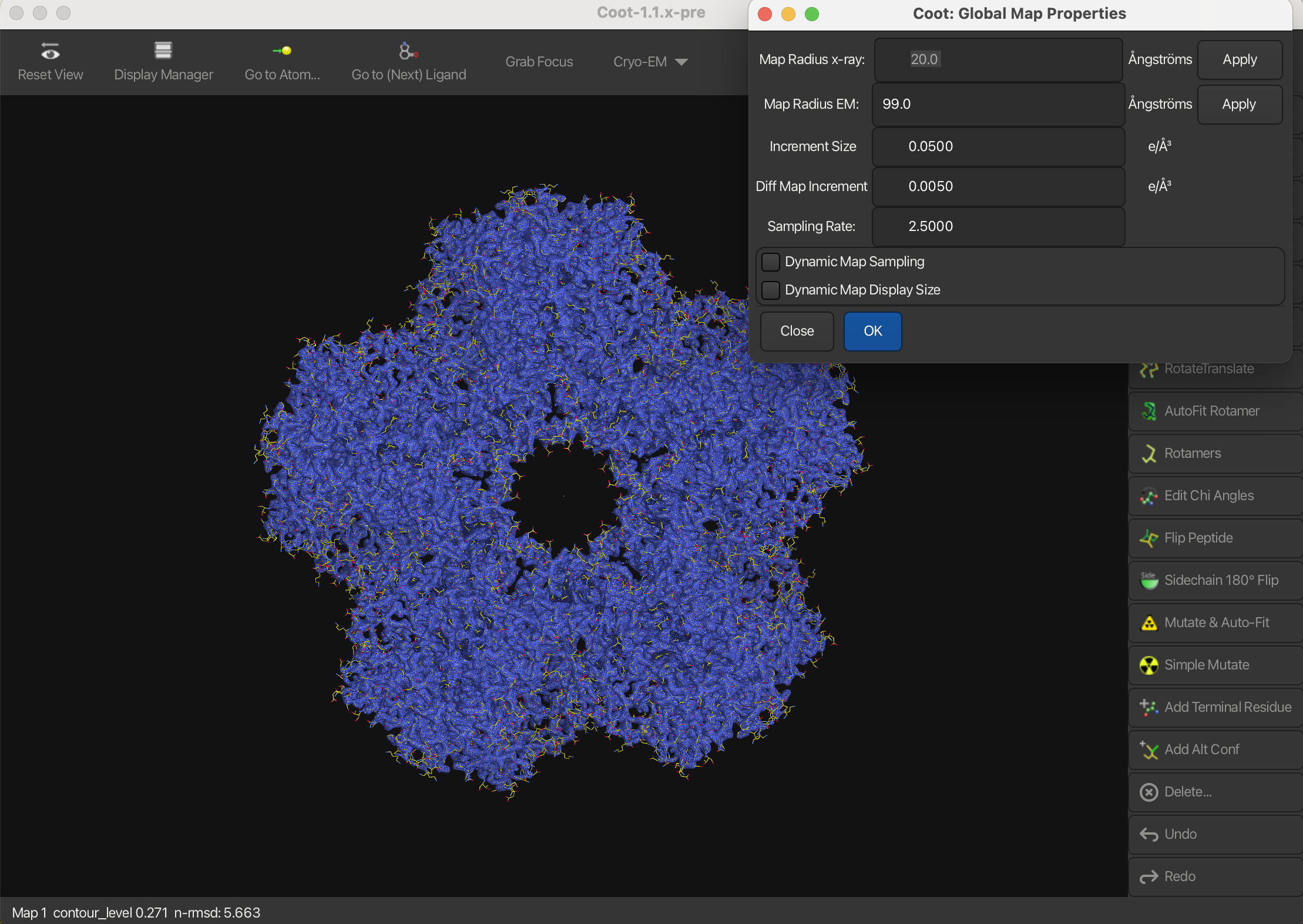
Let’s increase the radius:
- Navigate to Draw → Molecule → Map Parameters.
- In the window that appears, adjust the Map Radius EM to 99 and press Apply.
- Press OK to close the window.
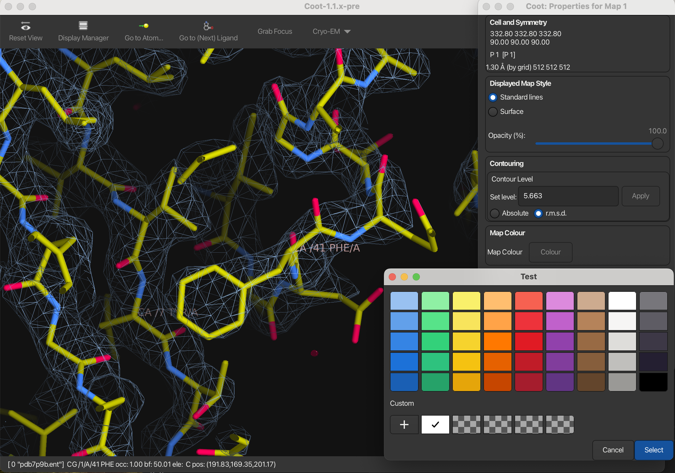
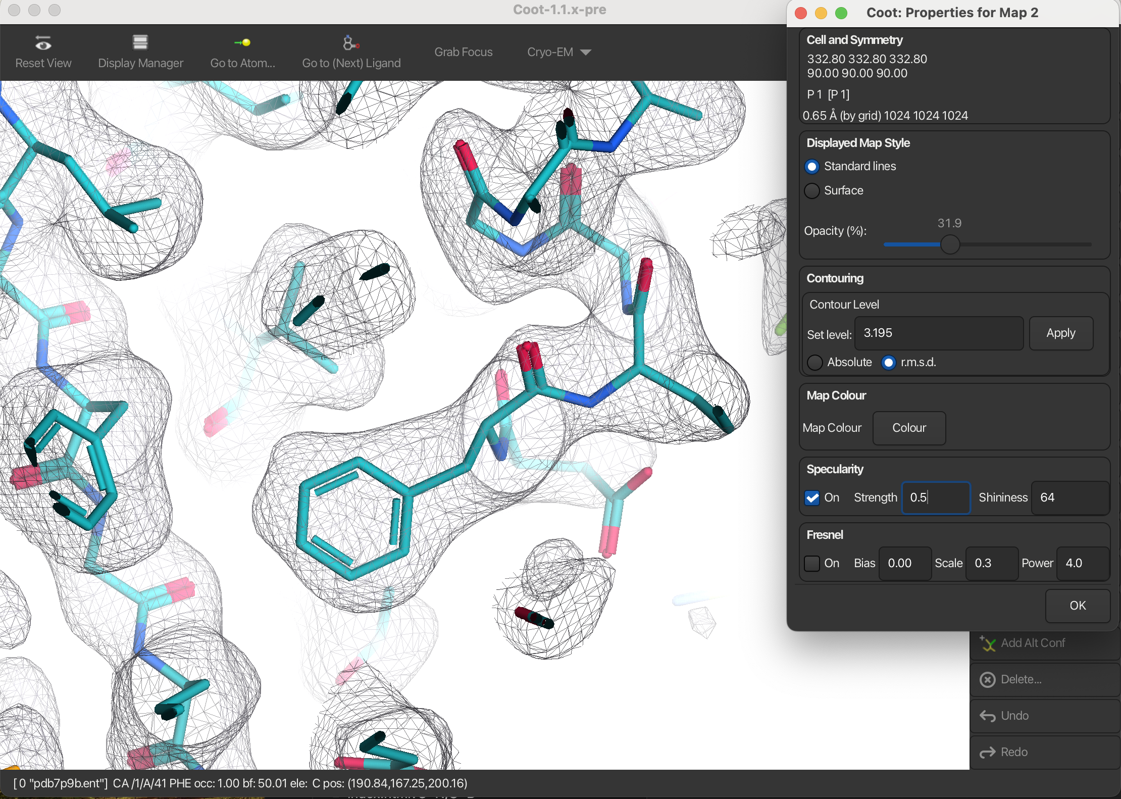
Colors
To change the color of the map:
- Open the Display Manager.
- In the Map window, select Properties. A new dialog will appear.
- Click on Map Colour.
- Click the + button to open the color picker and select a new color.
- Choose the desired color and press Select.
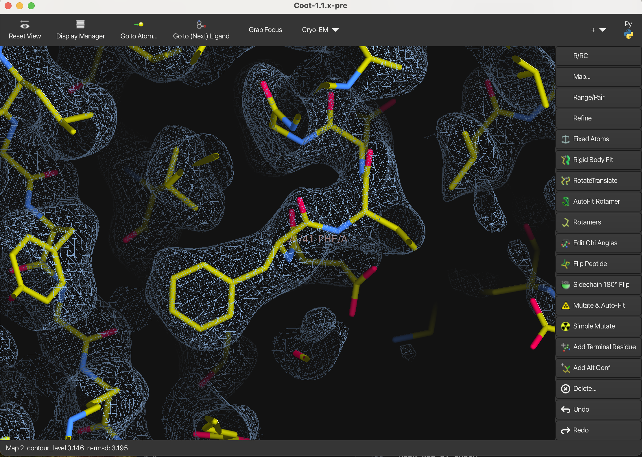
Smoothen
To make a smooth map:
- Navigate to Calculate → Map Tools → Make a Very Smooth Copy.
- Select the map you want to smooth and press OK.
This process may take some time depending on the size of the map. Once the new map is generated, it is recommended to avoid displaying both maps simultaneously to prevent visual clutter:
- Open the Display Manager.
- Undisplay or delete the original map.
Publication Tip
- Set the background color to white:
- Navigate to Draw → View → Background Colour and select white.
- Adjust the map color to grey:
- Open the Display Manager, go to Properties, and change the Map Colour to grey.
- Modify the map opacity:
- In the Properties dialog, adjust the Opacity slider to your preference.
- Fine-tune the clipping planes:
- Use the keyboard shortcuts 3 and 4 to adjust the back clipping plane, and 1 and 2 to adjust the front clipping plane, until the desired view is achieved.
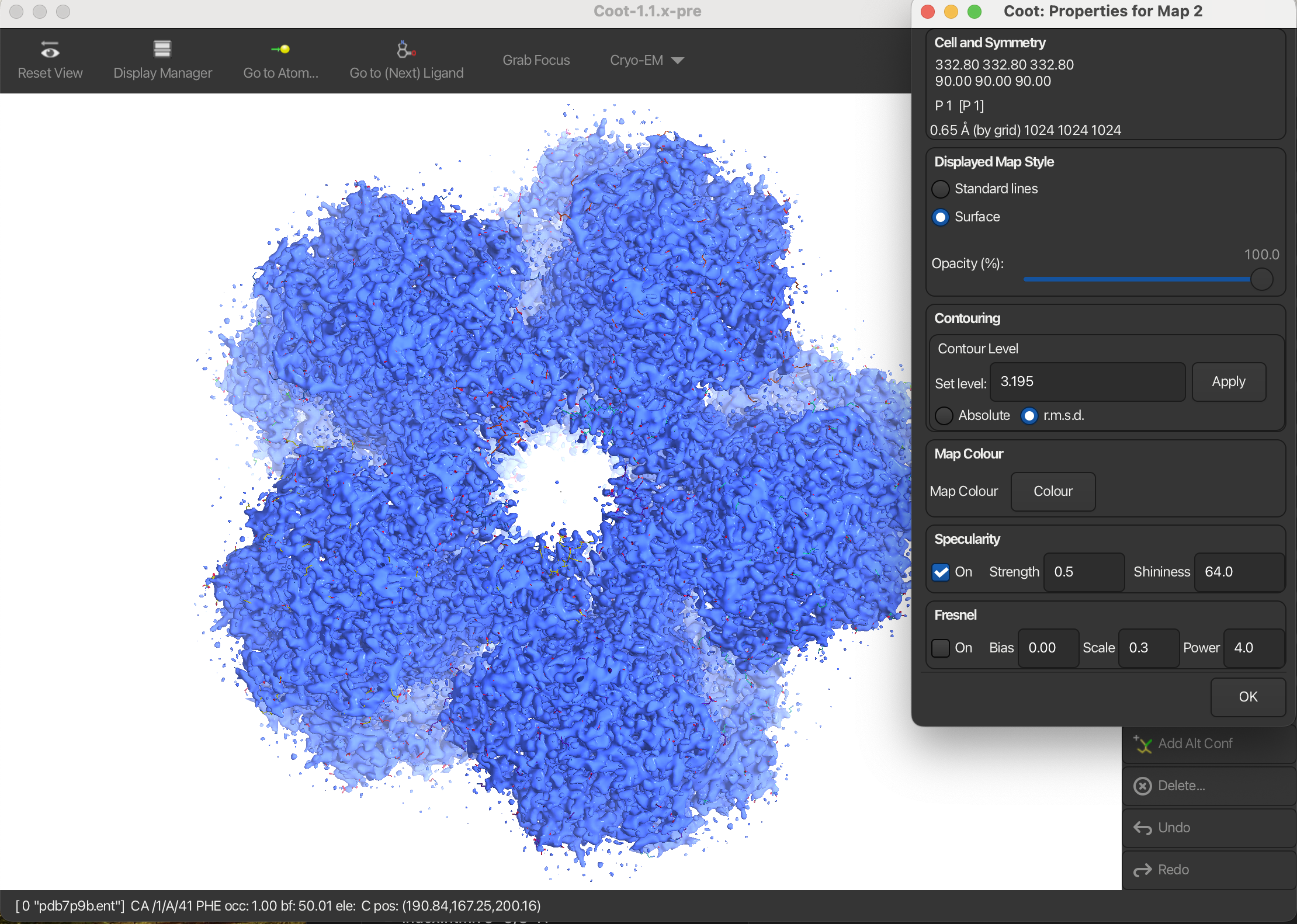
2.2 Surface
To create a surface representation of the map:
- Open the Display Manager.
- In the Map window, click on Properties.
- In the dialog that appears, set the Displayed Map Style to Surface.
This will render the map as a surface representation.
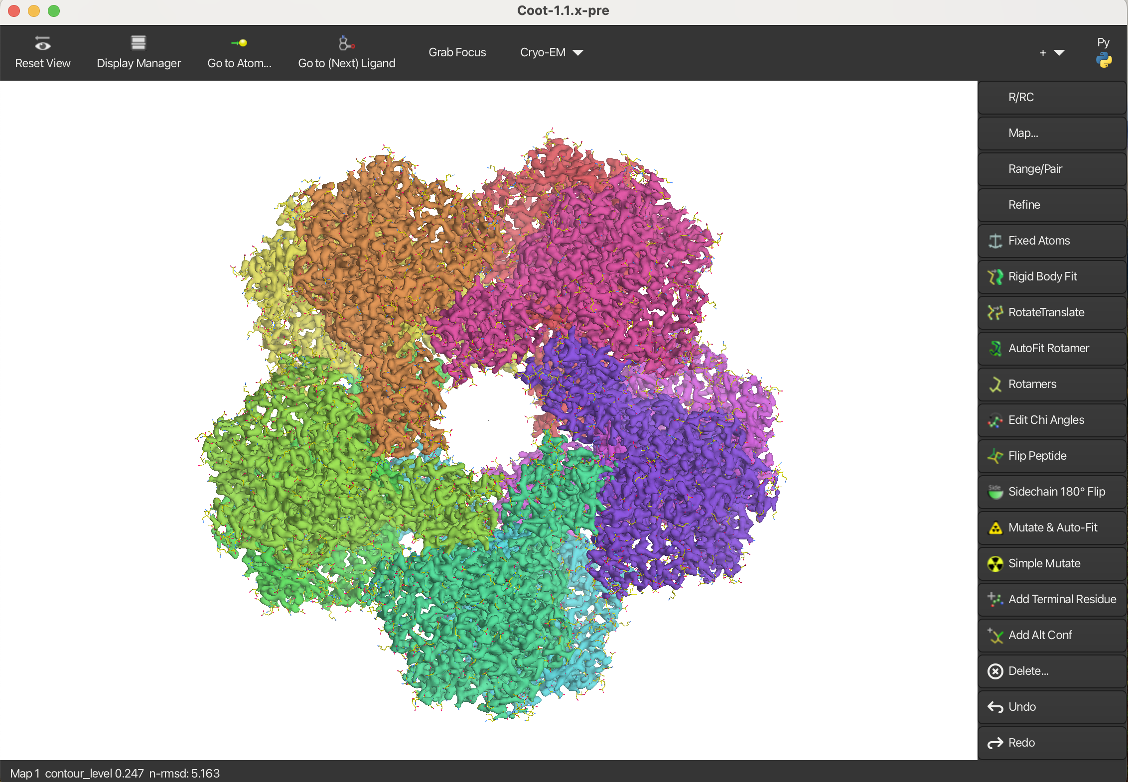
2.3 Mask the map
Mask map by chain
To mask the map by chains, follow these steps:
- Load the Cryo-EM module:
- On the right-hand side, click the button with a plus sign and an arrow.
- From the dropdown menu, select Cryo-EM. A new button will appear on the horizontal toolbar.
- Use the Cryo-EM → Mask Map by Chain option:
- Click the newly added Cryo-EM button on the toolbar.
- Select Mask Map by Chain from the menu.
The program will generate 10 new maps, each corresponding to one of the chains in the model. By default, these maps are displayed as chickenwire. To convert all maps to surface representations:
- Go to Cryo-EM → Solidify Maps.
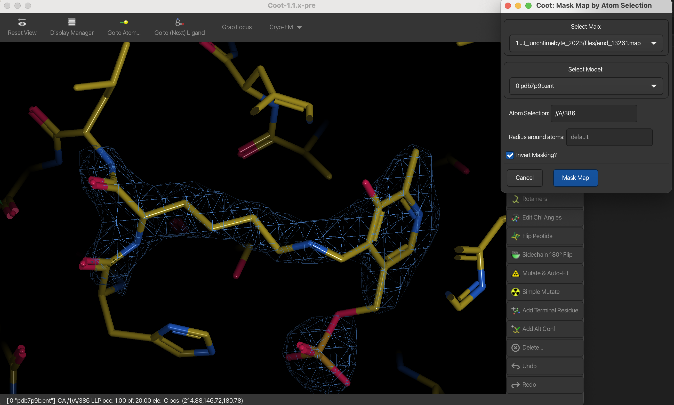
Mask map by atom selection
To mask the map by atom selection, such as for a ligand, follow these steps:
For example, we want to mask the map around LLP of chain A.
- Navigate to Calculate → Map Tools → Mask Map by Atom Selection.
- In the dialog that appears:
- Select the map you want to mask.
- Select the model.
- In the Atom Selection dialog:
- Specify the ligand details using the format
//A/386, which represents residue 386 in chain A (LLP). - Set the desired radius around the atoms.
- Check Invert Masking .
- Specify the ligand details using the format
- Press Mask Map to generate the masked map.
This process will create a new map focused on the selected ligand.
3. Shader Settings
3.1 Background
To change the background color:
- Navigate to Draw → View → Background Colour.
- Choose from various shades of grey, white, or black.
3.2 Clipping Planes
To adjust the clipping planes:
- Use 1 and 2 to modify the front clipping plane.
- Use 3 and 4 to modify the back clipping plane.
3.3 Lighting
To adjust the lighting settings:
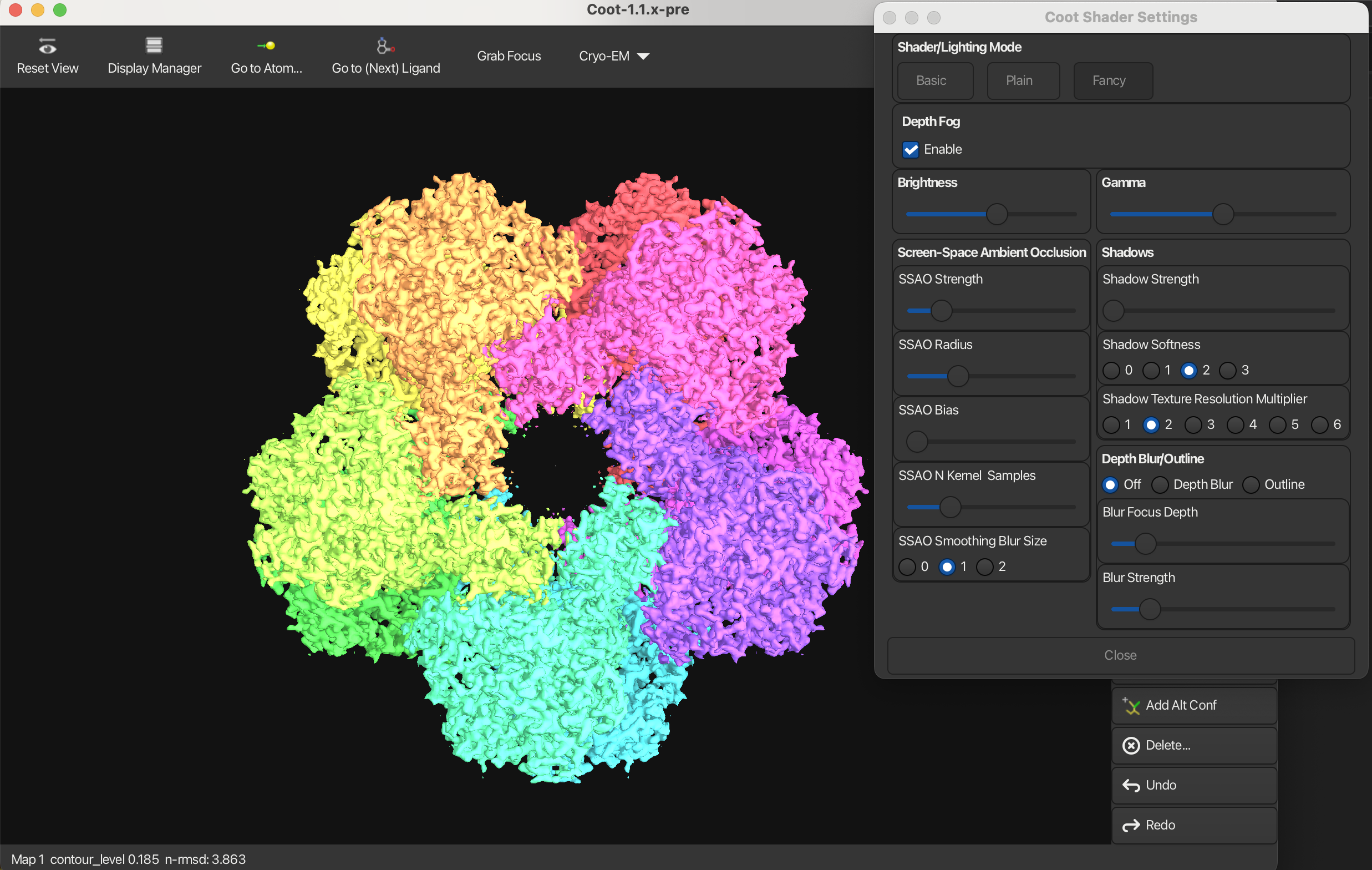
- Navigate to Draw → Shader Settings to open the Shader Settings window.
- Choose from the following modes:
- Basic: The default mode with standard lighting.
- Plain: Similar to Basic but with minimal shading.
- Fancy: Enables advanced shading and lighting options for enhanced visualization.
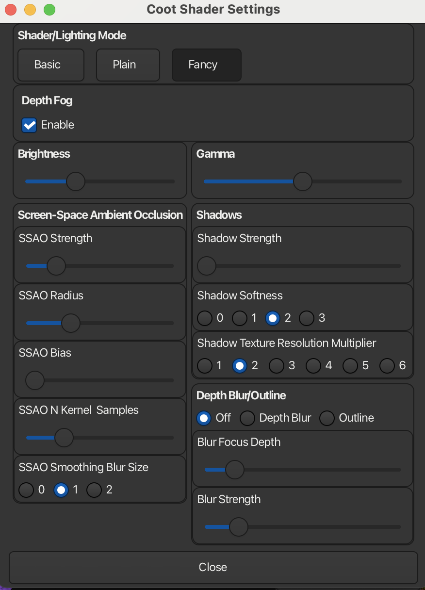
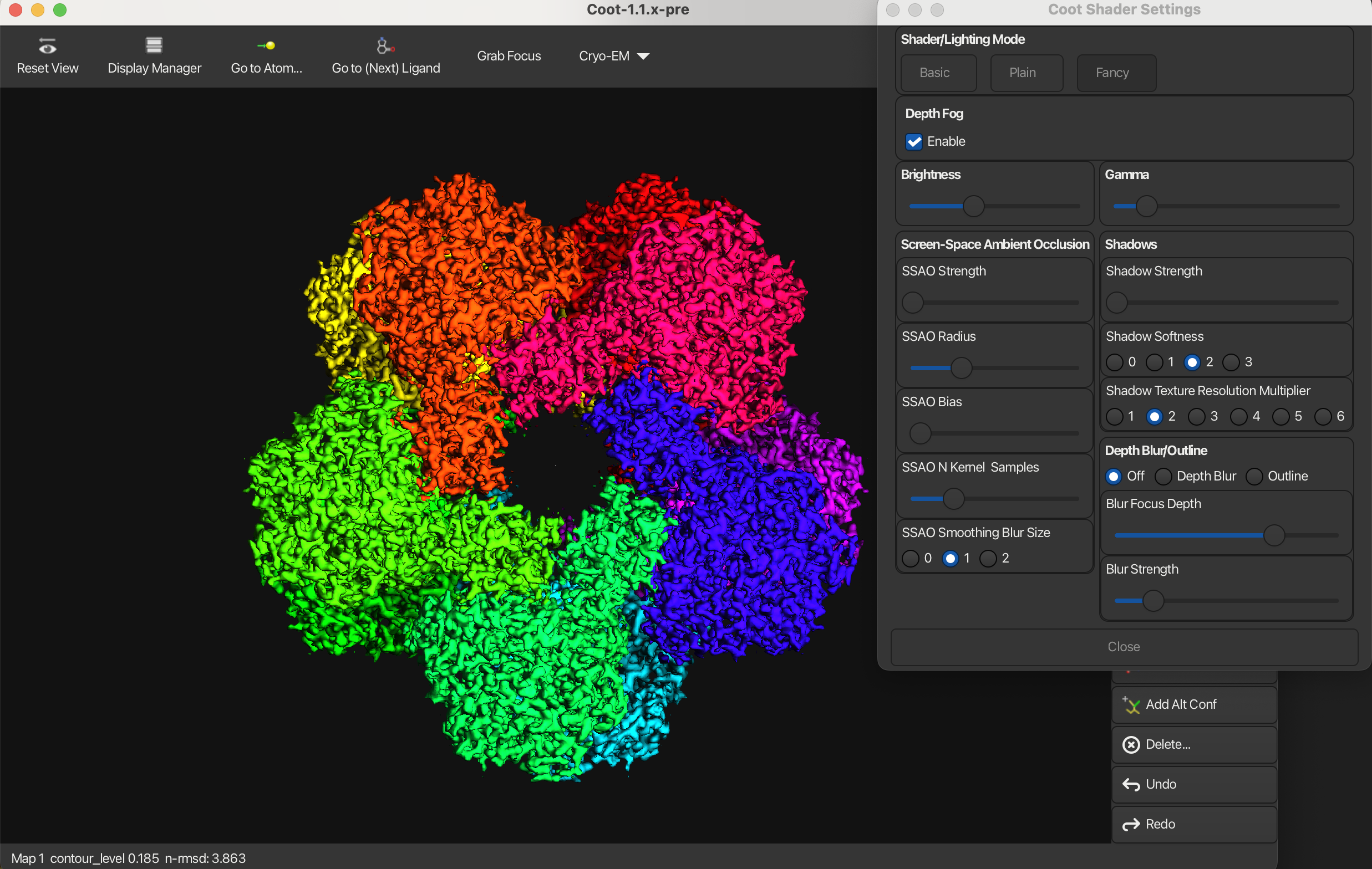
Fancy Mode:
Brightness
You can increase and decrease the brightness of the model by adjusting the Brightness slider.
Gamma
Adjusting the gamma setting can make the model appear more pastel and brighter when increased, or more vibrant and saturated when decreased.
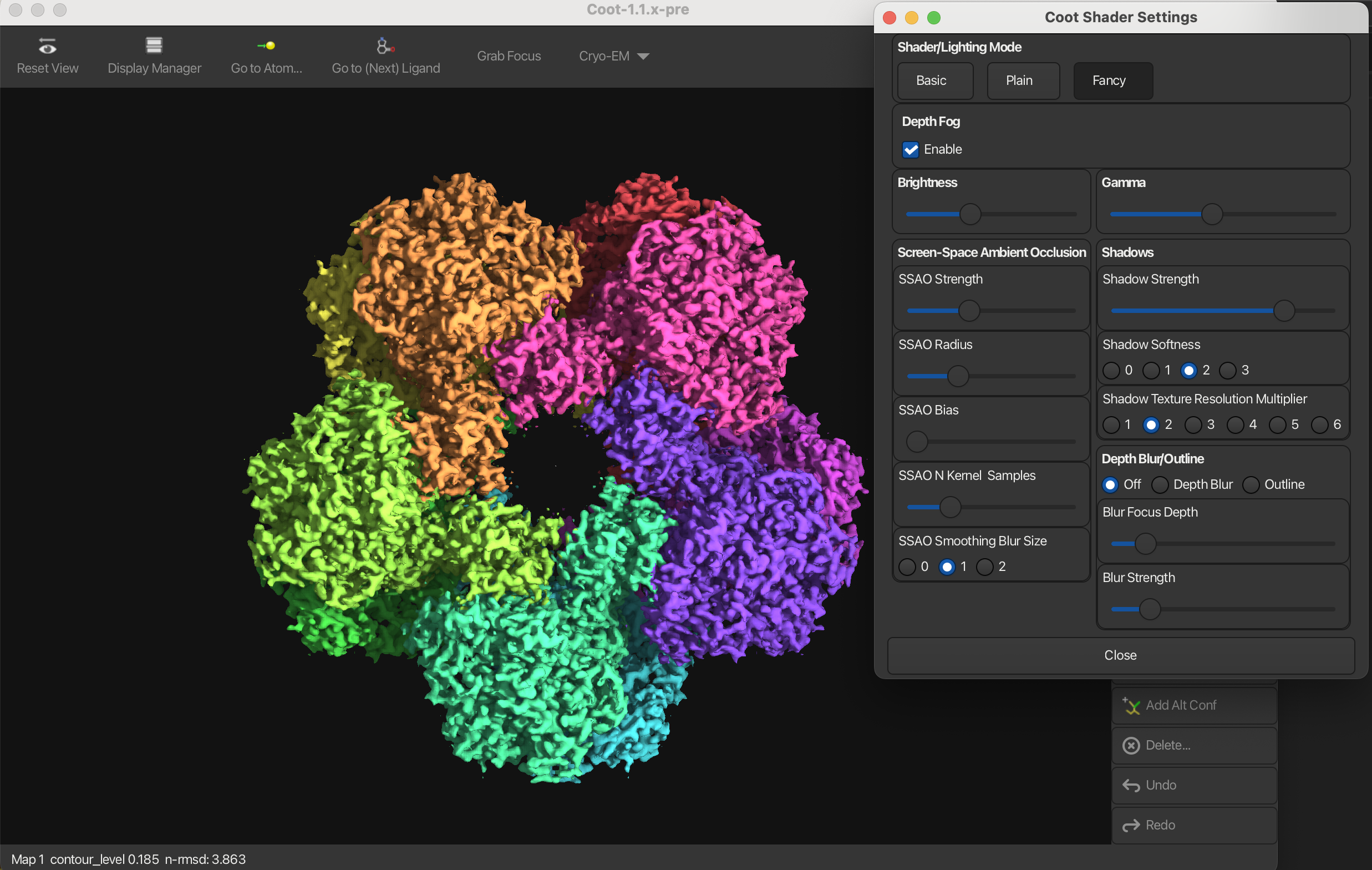
Screen-Space Ambient Occlusion
It is used to enhance the perception of depth and highlight cavities by simulating the way the light interacts with surfaces in a 3D environment. You can change the SSAO parameters such as the radius of the occlusion and the intensity of the effect. For high quality images turn up the kernel samples to the maximum.
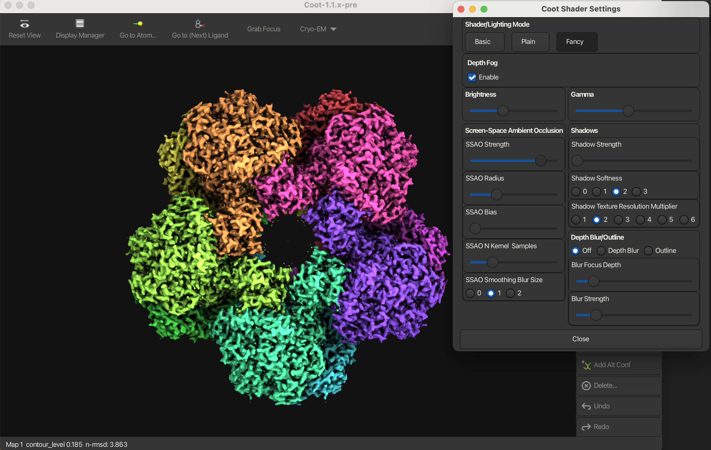
Shadows
Shadows can be enabled or disabled in the Shader Settings window. When enabled, shadows will be cast by the model, enhancing the 3D effect. This can be used in combination with SSAO.
Depth Blur
Depth blur is a feature that simulates the effect of a camera lens, where objects at different distances from the camera appear blurred. You can adjust the blur focus depth and strength to control the intensity and range of the depth blur effect.

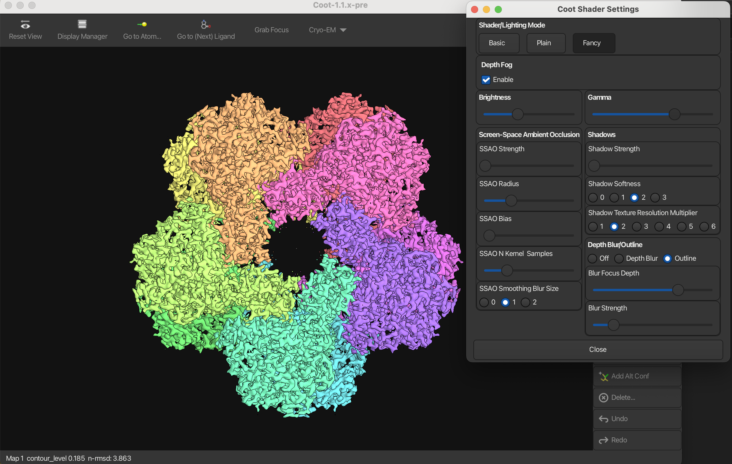
Outline
You can draw an outline around the model by checking the Outline box in the Shader Settings window.
4. Screenshots
Currently, the screenshot function is unavailable on some systems (including macOS) due to limitations with OpenGL support. The OpenGL screenshot feature requires OpenGL 4.4.
To capture screenshots, users are advised to use a third-party tool such as:
- macOS Screenshot Tool: Press Command + Shift + 4(or 5) to capture a selected area or Command + Shift + 3 for the entire screen.